Google Analytics on the Internet
Google Analytics (GA) is one of the most pervasive web analytics tools available on the Internet. Just how pervasive is it? 65% of the top 10k sites, 63.9% of the top 100k, and 50.5% of the top million use Google Analytics. In practical terms, this means that you're basically either on a website that is using Google Analytics or your next click will likely land you on one that does.
While the percentage of websites using Google Analytics has been calculated for the top N thousand websites, this is not a true measure of how widely the impact is felt. If you land on a web page with Google Analytics, a multitude of details are recorded, including the HTTP referrer, or web page that lead you to the current website. Thus, if you are unlucky enough to land on a web page using Google Analytics every second link click, Google might have enough information to reconstruct your entire path.
This line of exploration motivates our questions and the tasks required to answer them.
- What percentage of web pages on the Internet use GA for tracking their web traffic?
- If clicking a link from host A to host B, what is the probability that neither, one, or both pages have GA?
- If clicking a random link on the Internet, what is the probability that neither, one, or both pages have GA?
The NSA and Google Analytics
It has recently come to light that the NSA used (and may still continue to use) Google Ads and Analytics cookies to track users across the Internet. If you are on a web page that uses Google Analytics and the web page uses HTTP, the Javascript request and response, as well as the cookies that go along with it, are sent in the clear. If the unencrypted request is intercepted by a passive man in the middle (see NSA telecommunication interception facilities such as Room 641A), then all of this information is transparently available to the intercepting party. Most importantly, the Google Analytics cookie stores a tracking token that ties the session to a specific user. By intercepting and recording this information, it is alleged that the NSA are able to track the specific path that a given user may take across the Internet with the same level of knowledge as Google itself.
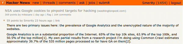
In the Hacker News comment thread where we discussed this new revelation in regards to our research, our comment was voted to the top of the page and sparked an extensive discussion. Two separate parties have emailed us specifically asking to be informed of the final results of our work.
The Common Crawl dataset
The first and most obvious question is, for a task that would involve such a large portion of web data, where do you acquire this? Crawling hundreds of millions of pages yourself is impractical in many ways and would be a substantial undertaking. Worst, this undertaking would take the majority of your time and yet not actually help answer the question directly.
Luckily, the Common Crawl Foundation is a non-profit foundation dedicated to providing an open repository of web crawl data that can be accessed and analyzed by anyone for free via Amazon S3. In total, the Common Crawl dataset consists of billions of web pages taken over multiple years, from 2008 to 2013. It has been used by a variety of projects, including commercial, academic, and even hobbyist projects.
The dataset is available in three different formats:
- Raw content retrieved via the HTTP requests (includes many file formats including HTML documents, PDFs, Excel, ...)
- Extracted textual content from the HTML pages found in the raw content
- Metadata from each of the HTTP requests. For web pages this includes extracted links, HTTP headers, reported character set, etc.
Common Crawl data is big data
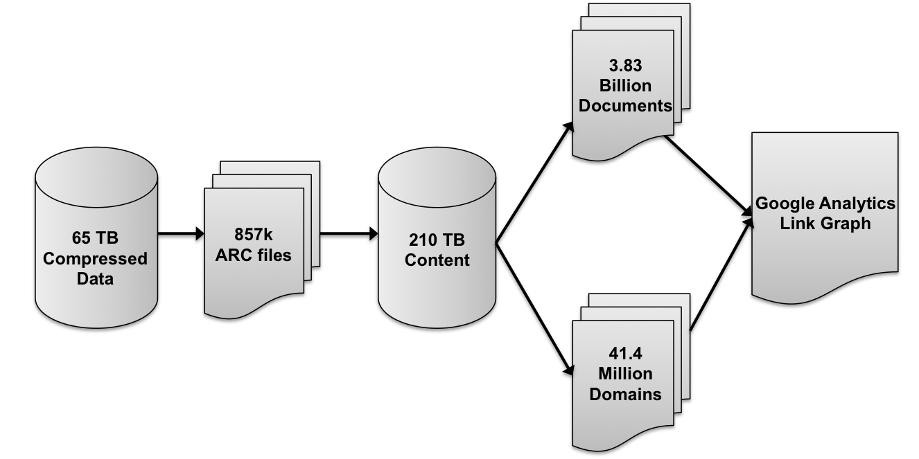
The 3.83 billion web documents of the 2012 Common Crawl dataset are stored on Amazon S3, split across 857,000 ARC files. Even when compressed using gzip compression, the total file size is quite substantial.
- Raw content: 65 terabytes compressed or approximately 210 terabytes decompressed
- Metadata: 40 terabytes compressed or approximately 126 terabytes decompressed
As a comparison, 210 terabytes of standard definition video (350MB for a 42 minute show) would allow you to store over 50 years of content!
Task Specifics
For our task, we need to produce two quite separate datasets: the Google Analytics count and the link graph. The link graph allows us to see when page A links to page B. The Google Analytics count tells us whether a given page uses Google Analytics.
To get an idea of the output size we were looking at, we looked at a comparable project, the Web Data Commons Hyperlink Graph. The graph is the largest hyperlink graph that is available to the public outside companies such as Google, Yahoo, and Microsoft. To enable for practical analysis, they offer the graph at multiple levels of granularity.
| Graph | #Nodes | #Arcs | Index size | Link graph size |
|---|---|---|---|---|
| Page Graph | 3,563 million | 128,736 million | 45GB compressed | 331GB compressed |
| Subdomain Graph | 101 million | 2,043 million | 832MB compressed | 9.2GB compressed |
The page level graph records all links from page A to page B, where page A may look like www.reddit.com/r/funny/. As can be seen, even though it is far smaller than the original dataset, it is still over a terabyte when decompressed.
The subdomain level graph records all links from domain A to domain B, where page A would be simplified from www.reddit.com/r/funny/ to www.reddit.com. The index (or list of nodes) for the subdomain level graph is just 2% of the index for the page level graph, and the reduction for the link graph is similar.
As our work is only an approximation and working with the subdomain level graph is substantially more tractable, we produce and work over the subdomain level graph for our work. Given the proper resources, however, our code is trivially modified to run both the Google Analytics count and the link graph generation a page graph.
We would have liked to use this existing resource for our work, but unfortunately the subdomain level graph does not record the number of links between two given domains, only whether a link exists. This is too little data for our task.
Expected Output
Google Analytics Count
The Google Analytics count will have output where the key is both the subdomain and the "GA state" of a page, and the value is the number of pages with or without Google Analytics.
www.winradio.net.au NoGA	1
www.winrar.com.cn GA	6
www.winrar.it NoGA	55
www.winratzart.com GA	1
www.winrenner.ch GA	244
www.winrichfarms.com NoGA	3
www.winrightsoft.com NoGA	1
www.winrmb.com GA	2
www.winrock-stc.org GA	1
www.winrohto.com NoGA	1
Link Graph
The link graph will have output where the key is DomainA -> DomainB and the number of times a link is directed from domain A to domain B.
cnet-blu-ray-to-avi-ripper.smartcode.com -> free-avi.smartcode.com	1
cnet-blu-ray-to-avi-ripper.smartcode.com -> macx-free-idvd-video-converter.smartcode.com	1
cnet-blu-ray-to-avi-ripper.smartcode.com -> perfectdisk-12-professional.smartcode.com	1
cnet-blu-ray-to-avi-ripper.smartcode.com -> rip-blu-ray-to-avi.smartcode.com	2
cnet-blu-ray-to-avi-ripper.smartcode.com -> videosoft-cnet.smartcode.com	1
cnet-cnec-driver.softutopia.com -> acer-power-fg-lan-driver.softutopia.com	2
cnet-cnec-driver.softutopia.com -> www.softutopia.com	24
cnet-digital-music-converter.smartcode.com -> android-music-app-maker.smartcode.com	1
cnet-digital-music-converter.smartcode.com -> convert-drm-wma.smartcode.com	1
cnet-digital-music-converter.smartcode.com -> converter.smartcode.com	3
Final Result
To compute the final result requires merging these two datasets together.
For each DomainA -> DomainB in the link graph output, we need to lookup the GA and NoGA values for those domains from the Google Analytics count.
From this, we can provide a loose approximation of how extensively Google Analytics is involved in the links from DomainA -> DomainB.
Tools
Language and framework
To tackle this task, we decided to use the Hadoop framework with Java instead of Python as the implementation language.
The decision to use Java falls to two main reasons.
First, the Common Crawl Foundation provide multiple libraries for use in Java and Hadoop for processing the Common Crawl datasets, such as loaders for the ARC file format.
These are well tested and have been used for significant projects by other parties before us.
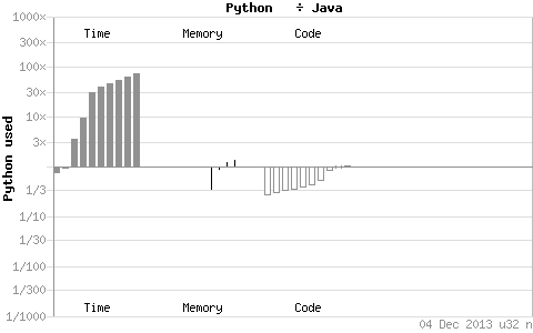
Second, while Python may be less overhead from a coder's point of view, Python is substantially slower than Java for the majority of general computing tasks.
This execution overhead is also exacerbated by mrjob, which allows for Python via Hadoop Streaming.
In this dataset, when efficiency is measured in both time and money, the performance losses that arise from Python are too substantial.
Development environment
Setting up a local development environment that contains Hadoop, the required libraries, and test data would be time consuming. To speed up the process, we use a virtual machine created for the Norvig Web Data Science Award, available here. The virtual machine comes set up with Oracle JDK 1.6, Hadoop 0.20.205, Pig 0.10.0, and Eclipse 3.7.2. With only minimal additional work, primarily setting up and installing Ruby and the Amazon EMR CLI, we have a fully operational development environment that allows us to test our code locally.
One minor issue is that some of the sample dataset provided with the virtual machine is out of date. This can be fixed by pulling down newer replacement files from Amazon S3.
AWS optimizations
For optimizing the cost of running this task, the primary avenue we can look towards is Amazon Web Services itself. In particular, we focus on spot instances, which allow for substantial savings on the computing hardware itself.
Spot instance considerations
To minimize the cost of our experiments, using spot instances on Amazon EC2 was vital. Spot instances allow you to bid on underused EC2 capacity, machines that would sit there unused otherwise. This allows you to utilize machines at just 10-20% of the standard instance price, allowing you to either spend less or to have far greater computing power for the same price.
The disadvantage with spot instances is that they can disappear at any time, either due to being outbid by others or as a result of high demand. Luckily, Hadoop is fairly resilient to transient nodes, though it can still result in a worse execution time.
Warning: Spot instances can actually exceed the standard cost of the machine. Do not set your maximum bid to more than you're happy to pay!
Selecting the optimal instance type
For our task, we are CPU bound, so want as much computing power as possible. We also don't need machines to exhibit any particular characteristics (such as "has GPU", "greater than N GB of RAM", ...), allowing us flexibility in machine choice. To work out which machine is the most cost effective, we took the average hourly spot instance price and divided it by the total number of EC2 Compute Unit (ECUs) the machine has. A single ECU provides approximately equivalent CPU capacity to that of a 1.0-1.2 GHz 2007 Opteron or 2007 Xeon processor. While this is not an exact measure of the machine's performance, it is representative.
From our analysis, we found the two most competitive instances are both from the previous generation of compute optimized instances, the c1.* family. This isn't surprising, though it is surprising that the current generation compute optimized instances are not competitive pricewise at all. This is likely as there are less of the current generation instances on EC2, resulting in higher competition for the current generation compute optimized spot instances. The High-CPU Medium (c1.medium) has 5 ECUs distributed amongst 2 cores while the High-CPU Extra Large (c1.xlarge) has 20 ECUs distributed amongst 8 cores.
| Machine | ECUs | Hourly spot instance price | Price per single ECU |
|---|---|---|---|
| c1.medium | 5 | $0.018 per hour | $0.0036 per hour |
| c1.xlarge | 20 | $0.075 per hour | $0.00375 per hour |
While the optimal instance appears to be the c1.medium, there are two things to consider. First, the standard fluctuations in the spot instance price means that the c1.xlarge can become the most competitive instance. Second, to get the same computing capacity as a c1.xlarge, we need to launch four times as many c1.medium instances. This adds a large amount of overhead, both in terms of spinning up and configuring the EMR cluster and also for the master to actually manage the cluster during the task.
Due to the lower accounting overhead and near comparable price, we decided on using the c1.xlarge instances.
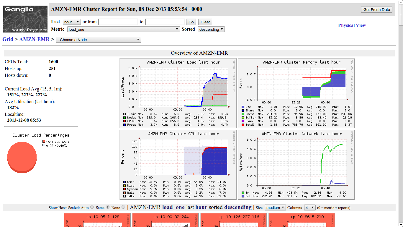
Spot instance availability
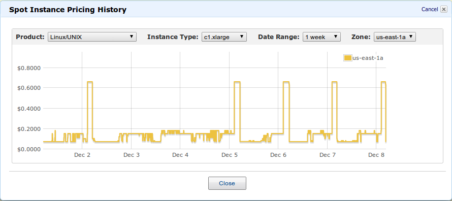
The price of the spot instances fluctuates similar to a stock market. If demand is high, expect to pay more for the resource. If demand is low, you might snag yourself a deal. As the price is related to demand, other jobs run on Amazon EC2 can impact how much you need to pay at a given time. Below, we can see the fluctuations in price for the c1.xlarge instance. Of particular interest, between 9pm and midnight many evenings, it appears someone runs a massive job that uses up almost all the spare capacity. Numerous times we have had to postpone our jobs or more to different Amazon regions in order to run a job at a reasonable cost.
Elastic MapReduce (EMR) overhead
One unfortunate consequence of using Amazon's Elastic MapReduce (EMR) is that there is a cost overhead applied to each instance that is part of the EMR cluster. This cost overhead is commonly more expensive than the machine itself when using spot instances. If hundreds (or even dozens!) of these styles of jobs are to be run, it would make sense to construct your own Hadoop cluster instead of relying on Amazon EMR to do it for you.
This might appear extreme, but it would literally result in a 50% or more reduction in the cost of the task.
| Machine | On-demand instance price | Hourly spot instance price | Hourly EMR management price | EMR as percentage of spot instance price |
|---|---|---|---|---|
| c1.medium | $0.145 per hour | $0.018 per hour | $0.030 per hour | 166% |
| c1.xlarge | $0.58 per hour | $0.075 per hour | $0.12 per hour | 160% |
Hadoop optimizations
The majority of the expense in this task is in executing the mapper and reducer code. As such, optimizing this part of the code is essential. To evaluate how the proposed optimizations impacted the efficiency of our task, we ran multiple experiments on a small subset of the Common Crawl dataset. This subset is 1/177th of the Common Crawl dataset, or approximately 1TB of data. The cluster used in this experiment consisted of 12 c1.xlarge spot instances as workers and a single c1.medium as the Hadoop master node.
Combiner (in-mapper reducer)
A combiner is similar to a reducer except run on the mapper before the data is sent across the network, hence why it is also called an "in-mapper reducer". By running a reduce task before sending the data across the network, the output size of the map step can be reduced substantially. This minimizes the network traffic between machines and also means the reduce step has to do less work. As there are commonly more mappers than reducers, this can also mean more computing power can be used, especially for the early stage of the reduce task.
Compression
At the end of both the Map and Reduce stage, we can use compression to reduce the size of the given stage's output, reducing the network and storage usage. This does come at a trade-off however, as compressing and decompressing the data leads to overhead for the task.
In our experiments, we use the Google Snappy algorithm at the mapper stage and the slower but more efficient gzip algorithm for the final output. Google Snappy does not aim for maximum compression, but instead aims for very high speeds and reasonable compression. This minimizes the speed penalty for compressing the large amount of data during the mapper process but gives us the benefit of lower network usage.
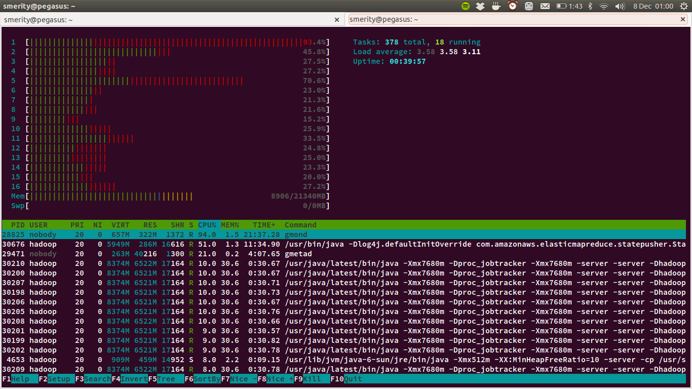
Re-using JVMs
It is well known that spinning up a new Java virtual machine (JVM) is time intensive. By default in Hadoop, a new map task is spun up after processing only 20 inputs. As there are 857,000 input files for the full Common Crawl dataset, that means there are over 42,000 JVM restarts.
More important than this, the JVM restarts result in lost optimizations for the code. This is as the JVM continually analyzes the program's performance for "hot spots", or frequently executed code snippets. These code snippets are then further optimized through just-in-time (JIT) compilation, leading to better performance. Each time a JVM is restarted, these "hot spot" optimizations are lost.
Increasing total mapper jobs
By default, Amazon EMR optimizes the number of mappers to be equal to the number of CPUs the given machine has. While this would be the correct choice for many tasks, it leads to suboptimal performance in our situation.
Our task is not IO bound, but retrieving the next data segment from Amazon S3 takes both time and bandwidth. This can result in too little work for the CPU when finishing a map process until the next one starts. By over-utilizing the CPU by adding additional mapper tasks, the CPU will always have a new segment of data to work on, as the input file will already have been buffered.
Over-utilizing the CPU traditionally results in worse performance in many tasks due to cache thrashing. This is quite a specific situation.