

Overview
Stochastic ray tracing is one of the fundamental algorithms in computer graphics for generating photo-realistic images. We implement an unbiased Monte Carlo renderer as an experimental testbed for evaluating improved sampling strategies. Our results show that the improved sampling methods we use for rendering can give comparable image quality over twenty times faster than naive Monte Carlo methods.
Approach
To simulate the global reflection of light throughout a scene, we need to consider how light moves around the scene. This is referred to as the light transport equation, described in Kajiya (1986). The basic idea is light is either produced by the object (emission) or reflected onto it from other objects (reflected). For full details, refer to our paper.
\begin{align} L_{out}(x, \theta_o) & = L_{emit}(x, \theta_o) + L_{reflected}(x, \theta_o) \\ & = L_e(x, \theta_o) + \int{L_i(x, \theta_i) f_r(x, \theta_i, \theta_o) | \theta_i \cdot N_x | \partial w_i} \\ & = \text{emitted from object} + \text{reflected onto object} \end{align}
The integral for the reflected light is computed over the hemisphere of all possible incoming directions. As this is impossible to compute exactly, it is approximated using Monte Carlo methods. The primary issue that can occur is when noise is too strong to give reasonable estimations as to the radiance. Whilst the expected value remains accurate, the standard deviation (error) decreases by $\frac{1}{\sqrt{n}}$, where $n$ is the number of samples. To achieve a noise free image requires a large number of samples, especially if the scene is complex.
Importance sampling using BRDF sampling
Some materials only reflect light in very specific directions. This is commonly related to the roughness of the material. A mirror, such as the one on the left, needs far less samples than the diffuse surface on the right.
This is dictated by the material's Bidirectional Reflectance Distribution Function (BRDF). This distribution function dictates how much light ends up reflected in a given direction. By sampling directions to test directly from this distribution function (importance sampling), we can avoid taking samples that contribute little to the final image.
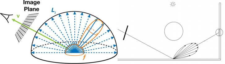
Uniform sampling of the potential bounce directions (blue) versus BRDF sampling (orange).
Importance sampling using explicit light sampling
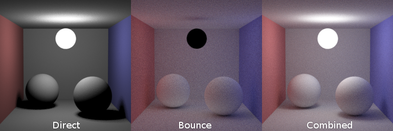
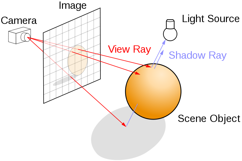
In an unbiased Monte Carlo renderer, the light path being sampled must hit a light source (luminaire) before it can make any contribution to the radiance of a given pixel. When the luminaire is small, the probability that a random light path will intersect with it is highly unlikely, requiring a larger and larger number of light paths to be sampled. By exploiting our knowledge of the scene, specifically the location of these light sources, we can perform importance sampling towards their locations. By sampling towards the light and checking if any other objects intervene (a "shadow ray"), we don't need to wait for chance to point us to our strongest light contribution in the scene.
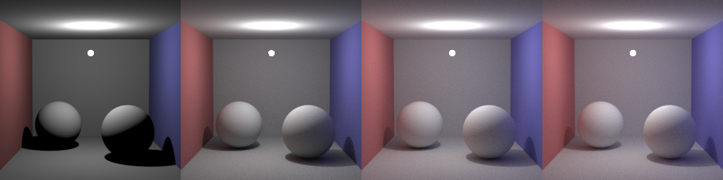
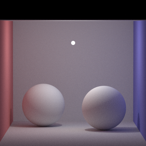
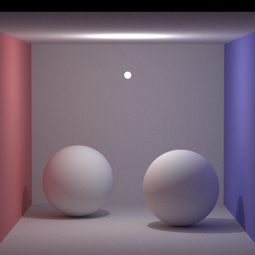
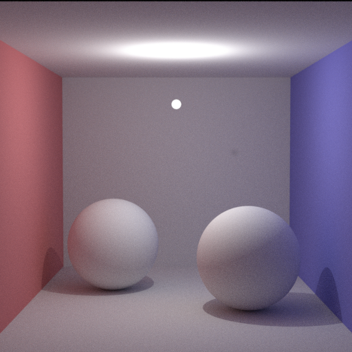
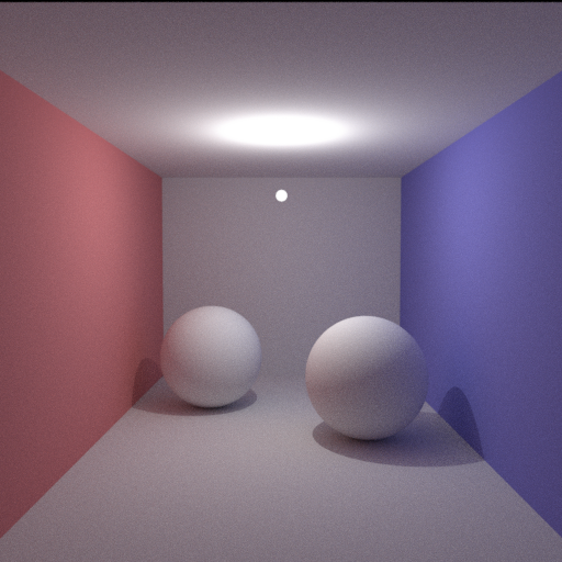
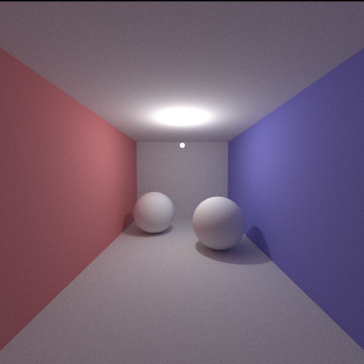
In the two animated images below, we can see the impact that explicit light sampling has on rendering. The animated image that does not use explicit light sampling begins almost completely black, adding speckled light over time. This is as the majority of light paths never end up at the small light source.
The animated image with explicit light sampling is comparatively boring. Even at the very start, the majority of the scene is well defined. Whilst it does have noise, the noise is close to the eventual value rather than being black, as in the previous image.
The most important thing to realize is that the image on the left shows one frame per 50 samples, whilst the image on the right uses one frame per sample. As such, the image on the left is shown at approximately ten times real rendering speed whilst the image on the right is near real time.
The image on the left uses 2,500 samples per pixel, no explicit light sampling, and takes 10 minutes to render.
The image on the right uses only 50 samples but performs importance sampling using explicit light sampling, and renders in 10 seconds.
Rejection sampling via Russian roulette path termination
Bright photons in real life may bounce millions of times, but computing such a long path is intensive and contributes little to the final result. Stopping after a finite number of bounces can result in significant bias however.
Instead, we introduce Russian roulette path termination, where at each bounce we terminate the light path with probability $q$. This probability is selected proportional to the overall reflective properties of the material. This means bright objects encourage more bounces whilst dark objects encourage less. As dark objects absorb more light, this means that terminating the path early is unlikely to increase the noise in the image.
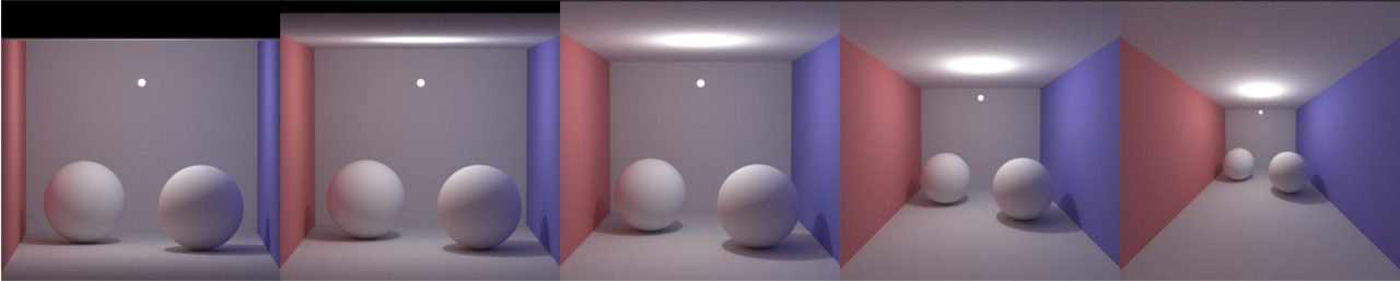
The first three images have a maximum allowed light path length of 1, 2, and 3, taking 18 seconds, 31 seconds and 58 seconds respectively.
The image on the right uses Russian roulette path termination, taking 83 seconds.
Whilst in our scene, extreme bias can primarily be seen in images of maximum allowed light path length of 1 and 2, extreme bias can still be visible in more complex scenes even with max depths of 10 or more.
Variance reduction
Monte Carlo raytracers traditionally work by taking a specified number of samples for every pixel in the image. Though this is guaranteed to produce a desirable result for large enough $n$, it can lead to substantial computational effort being spent on pixels that do not require any additional samples.
Motivated by this understanding, we implemented adaptive sampling, which would perform sampling over the pixels according to rejection sampling of the perceived variance. The perceived variance is defined either by the variance of the individual pixel or the expected variance when compared to neighbouring pixels. Unfortunately, we found that the large amount of overhead required to perform these calculations is less efficient than simply performing more samples. Whilst the results produced were of comparable quality, the overhead necessary to store all the samples stored was too large to be offset by any of our computational gains.
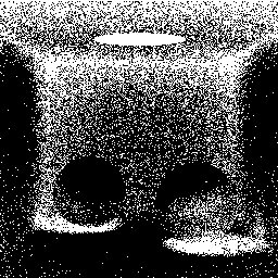
The accompanying image displays the relative variances of the pixels in the image, with pixels of higher variance colored darker than those of lighter variance.
Here the variance was measured solely based on the history of the individual pixels.
Simulating physical phenomena
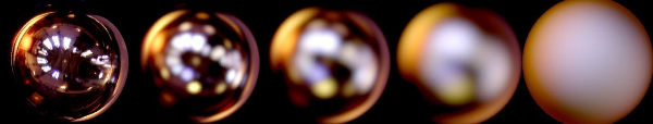
Monte Carlo methods allow easy emulation of physical phenomena such as camera lenses, including aperture size and focal length. This can be extended to other physical phenomena including motion blur, which is simply performing Monte Carlo sampling over time as well.
Impact of various focal lengths on the resulting image.
Note how the first few are "flat" whilst the latter ones appear stretched.
When we modify aperture size and focal length, we also modify how the camera samples pixels from the shot. For each pixel in our image, samples are taken over multiple rays, each sent at slightly different angles, all converging at the focal length. By using Monte Carlo sampling, we approximate sampling over all possible rays, resulting in a physically accurate blur in the foreground and background.
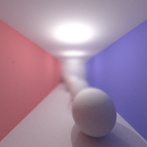
Exaggerated depth of field to emphasize the accurate blur produced by Monte Carlo sampling.
This can be combined with variance reduction such that more samples are taken in the less defined, blurrier parts of the image.